T+n time series analysis

This isn’t stock advice, it’s a data and math project. AAPL is interesting (not investing advice!) from a data perspective. Part of my big data project was the creation of a tool to analyze every symbol regressed on every other symbol for numerous lags. In addition to revealing the vendor’s mangling of data for unknown purposes, that analysis of lags produced at least one independent variable upon which the regression of future AAPL produced a .3 R-squared value. That is a weak or low effect size, but was a genuine discovery which passed hypothesis testing across time horizons. That was Direxion Daily S&P Oil & Gas Exp. & Prod. Bear 2X Shares (DRIP). DRIP was the first independent variable I discovered through the lag analysis. The problem is that the lag analysis is very computational intensive. Then, after doing that, ferreting out the red herrings because of bogus data takes another large amount of time. It seems that my data provider inserts bogus data producing .9 r^2 values between different vectors. These are of course problems that can one can mitigate with better code. That too, takes time. This isn’t a document about that first statistically significant predictor for AAPLt+3.

Keeping the t+ and t- in mind causes some difficulty for me. T+2 means today plus 2. If today is January 5, t+2 is January 7. If we are analyzing t+3, that is January 8. Programming in 0-indexed programming languages produced an inner impulse to count from 0 instead of 1. With zero indexing, the third option is 7 as shown in this example of a list [5, 6, 7, 8]. This is a heavily ingrained impulse that I must both use and mitigate. This project used Python and R and shell scripting.

The first 1 factor model devised using DRIP was as follows:

-2.065(DRIP Typical %change) -.0040 = AAPL Typical %changet+3

This model was tested in Stata using the data in manipulated in Python and R. This formula may be of no use in the future or even now. I might revisit this in discussing lags portion of the project later

Posted in Computing Notes | Tagged , , | Comments closed

Stata reference material

Linear regression analysis using Stata contains a look at Stata output for regression. There is also an excellent document on Regression Analysis | Stata annotated output at this link. There is an excellent document on Basic Data Analysis and Manipulation at this link. Yt−1 is the first lag of Yt (Chapter 10, p. 1).

Posted in Computing Notes | Tagged | Comments closed

Apple and Peach Goal Trees

I added an Apple tree to the planter that contains the peach tree.  This is a Red Delicious apple tree sprouting leaves for the spring.image
image

The Peach Tree looks good.  Here it is before the placement of the Apple tree.
image

Posted in Garden Notes | Tagged , , | Comments closed

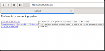
Rudimentary versioning system

Some time ago, Python 2 was the default language for use with Linux and Gnome 3. A set of extensions for Gnome, called Nautilus Python existed which allowed one to create customized right click menus. One of these was called “Historical Copy” and it created a lovely copy of the file with a timestamp inserted into the file name. The timestamp was constructed to allow the files to appear easily sorted when perusing directories. Software rot affects all software and especially software that requires Python 2 libraries that maintainers no longer ship on new versions of Linux. To counter this problem, we have a rudimentary versioning system which adheres to the Keep it Sweetly Simple (KISS) principle.

The following code is appended to the .bashrc file in the home directory.

### Historicaly copy rudimentary versioning system
### Saves a historical copy and a note about that copy
### Compressed to 68 character width for website display purposes

historicalcopy() { mkdir -p local-historical-versions &&\
 timestamp=$(date +"%y.%m.%d.%H%M") && read -p\
 "Enter filename:" n && read -p "Enter note: " note &&\
 filename=$(pwd)/$n && file_name=$(basename $filename) &&\
 left_side="${file_name%.*}" && extension="${file_name##*.}" &&\
 cp $filename\
 local-historical-versions/${left_side}-$timestamp.$extension &&\
 cp $filename\
 /var/www/html/hv/archives/${left_side}-$timestamp.$extension &&\
 sed -i "11i${left_side}-${timestamp}.${extension} ${note}"\
 /var/www/html/hv/index.php; }

From the directory with the file to be versioned, the command historicalcopy is typed.  This creates a directory in the current directory called local-historical-versions and copies the historical version into that directory.  It then copies the file to a complete historical versions archive and appends a PHP file in the web-server directory with both a link and comment.  The reason periods are used instead of dashes is because experience demonstrated that my software using Python had difficulty with filenames incorporating dashes.  This naming style is similar to the RPM naming convention which uses name-version-release.  This rudimentary versioning system uses a timestamp as the version number.  There are plenty of more advanced systems such as git, but sometimes we can work more efficiently with a simple direct historical list of what file did what way back when.  This could easily be changed so that an html file is updated in a local directory instead of a PHP file on a web-server.  The PHP file is future usage incorporated with user authentication and a long term code repository.  The code can then be used on OSX and Windows Subsystem Linux by pulling the PHP to the local machine, inserting the necessary file, and then transferring it back to the web-server via SSH.  In a way that seems like Git, but this is for the use case where one wants a simple to use list.

A typical workflow goes something like this.  Open up a terminal and navigate to the directory containing a heavily evolved r script.  Use the historicalcopy command on that script with a note something like “prior to adding the new data frame for time series data on Kentucky unemployment”.  Then open that file in the editor of choice to work on it.  It is very useful for Python programs where huge changes can take place which require significant removal of existing code.  This is the case for one of my projects which has been an ongoing project involving thousands and thousands of lines of code that has evolved over four years.  This simple scheme lets me remember which files had the important code that I still want to use in the future. The flat file format and easy naming convention allows easy migration, backups, and reduces the learning curve.

image

Posted in Computing Notes | Tagged , | Comments closed

Persistent Notification in Gnome 3

This is a GTK notification in Linux that remains on screen until it is clicked.

#!/usr/bin/python3

import gi
gi.require_version('Notify', '0.7')
from gi.repository import Notify
gi.require_version('Gtk', '3.0')

Notify.init("Hello world")
Hello = Notify.Notification.new("Hello world - the heading",
                                "This is an example notification.",
                                "dialog-information")

# https://www.devdungeon.com/content/desktop-notifications-linux-python
Hello.set_urgency(2) # Highest priority
Hello.show()

Last updated and tested 12 December 2020 on CentOS 8 (not Stream).

Posted in Computing Notes | Tagged , | Comments closed

Labeling variables in R

This great procedure makes it easy to remember what variables are related to in R. One of the troubles with exploratory data analysis is that when one has a lot of variables it can be confusing what the variable was created for originally.  Certainly code comments can help but that makes the files larger and unwieldy in some cases.  One solution for that is to add comment fields to the objects created so that we can query the object and see a description.  So, for example, we could create a time series called sales_ts, and then create a window of that, called sales_ts_window_a, and another called sales_ts_window_b, and so on for several unique spans of time.  As we move through the project we could have created numerous other variables and subsets of those variables.   We can see the details of those by using head() or tail(), but that may not be an extremely useful and clear measure.

To that end, these code segments allow applying a descriptive comment to an item and then querying that comment later via a describe command.

example_object <- "I appreciate r-cran."
# This adds a describe attribute/field to objects that can be queried.
# Could also change to some other attribute/Field other than help.
describe <- function(obj) attr(obj, "help")
# to use it, take the object and modify the "help" attribute/field.  
attr(example_object, "help") <- "This is an example comment field."
describe(example_object)

The above example refers to an example object, that could easily be sales_ts_window_a mentioned above.  So we would use the attribute command to apply our description to sales_ts_window_a.

attr(sales_ts_window_a, "help") <- "Sales for the three quarters Jan was manager"
attr(sales_ts_window_b, "help") <- "Sales for the five quarters Bob was manager"

After hours or days have passed and there are many more variables under investigation, a simple query reveals the comment.

describe(sales_ts_window_a)
[1] "Sales for the three quarters Jan was manager"

This might seem burdensome, but RStudio makes it very easy to add this via code snippets. We can create two code snippets. The first is the one that goes at the top of the file which defines the describe function that we use to read the field we apply to the comment to. Open RStudio Settings > Code > Code Snippets and add the following code. RStudio requires tabs to indent these.

snippet lblMaker
        #
        # Code and Example for Providing Descriptive Comments about Objects
        # 
        example_object <- "I appreciate r-cran."
        # This adds a describe attribute/field to objects that can be queried.
        # Could also change to some other attribute/Field other than help.
        describe <- function(obj) attr(obj, "help")
        # to use it, take the object and modify the "help" attribute/field.  
        attr(example_object, "help") <- "This is an example comment field."
        describe(example_object)

snippet lblThis
        attr(ObjectName, "help") <- "Replace this text with comment"

Now one can use the code completion to add the label maker to the top of the script. Simply start typing lblMak and hit the tab key to complete the code snippet. When wanting to label an object for future examination, start typing lblTh and hit tab to complete it and replace the objectname with the variable name and replace the string on the right with the comment. These code snippets provide a valuable way to store descriptive information about variables as they are created and set aside with potential future use.

This functionality does overlap with the built in comment functionality with a bit of a twist. The description added via this method appears at the end of the print output when typing the variable name. The built in comment function does not print out. It is also less intuitive than describe() and receiving a description.

R contains a built in describe command, but it often is not useful. Summary is the one I use most often. For a good description, I import the psych package and use psych::describe(data). Because of that, the describe method in this article is very useful. The printout appears like below with the [1]…

lu71802xbt90_tmp_dac5c795

Adding attributes other than “help” could easily be accomplished. DescribeAuthor, DescribeLocation, and other functions could be added. When using a console to program, a conversational style makes it flow better.

Posted in Computing Notes | Tagged | Comments closed

My Favorite Function

My favorite function of all time is varsoc in Stata.  That’s saying a lot because I have been working with computers for decades and have written software in several languages, used many different types of administrative software tool sets, and owned a lot of books with code in them.  Varsoc regresses one variable, y, upon another variable, x, and then regresses each lag of y on x to produce output that allows one to know the best fit lag for a regression model.   It allows someone analyzing time series data to immediately know that data from the several prior is a better predictor of today’s reality than more recent data.  I adore Stata for scientific analysis.  In order to use this for my big data project, I needed to automate it, and so I wrote an R vignette that would analyze 45 lags and produce the relevant test statistics. My vignette produces r2 values1, parameter estimates, and f-statistics for 45 lags of y regressed on x. The p-values are then written to a CSV file. The decision rule for a p-value is that we reject the null hypothesis if the p-value is less than or equal to α/2.2 The data comes from 5GB of CSV files that were created via Python.

Running the lags shows us the relationships between the historical prices of two securities. When we regress y on x in this case, we are regressing the price of security 2 on security 1. We then do this on a lag. The L1 of security 2 regressed on security 1’s L0. Then we regress L2 of security 2 on security 1’s L0. This occurs for 45 iterations. For example, we might find that the price of a gold ETF 44 days ago has the best relationship with the price of Apple stock today as compared to the price of that same gold ETF 12 days ago and even today. That’s an example only and not anything substantiated in the data. There will certainly be some spurious relationships. An ETF buying shares of Apple and then the same ETF’s fee going up the next month, for example. To mitigate this, the vignette uses the first difference of the logarithm so that the data is stationary. The CSVs are already produced so that unit roots are accounted for. This is a research project to identify what actually bodes well in other sectors. It runs on every listed security on the American exchanges. Every symbol is regressed on Apple. Every symbol is regressed on Microsoft, and so on. The data is stationary and unit roots are eliminated.

I initially began this project some time ago and at that time I stopped because it was going to take a solid month of continuous 12-core processing to accomplish the entire series. In retrospect, I should have let that proceed but there would have been a great tradeoff in that I couldn’t have played Roblox, The Isle, and Ark Survival Evolved with my daughter. Finally, I’ve got the research running on a new machine dedicated to that purpose. That machine uses an AMD Ryzen 5 3500 and NVMe SSD. The program is running on 6 cores in parallel. Previously, with the one month estimate, it was running concurrently on 12-cores of Westmere Xeon CPUs and storing the output in RAM instead of on an SSD. This will serve as an interesting test for the Ryzen since all six cores will be running at 100% for months on end. The operating system is OpenSuse Leap 15.2, the R version is 4.05, and the Python version is 2.7.18.

One of the reasons to write these articles is for my own memory. It gets older to remember as one gets older. These blog posts are essentially a public notebook to aid myself and others.


1  R2 is the coefficient of determination, which is the square of the Pearson correlation coefficient, r, the formula for which is ρ=β1(σx/σy), where β1 is the parameter estimate. ASCI and Unicode text does not have a circumflex, ^, on top of the β. For this documentation the objective is multiplatform long-term readability so an equation editor with specialized support for circumflexes is out of the question.

2  There is also the existence of the rejection region method. We reject the null hypothesis if the test statistic’s absolute value is greater than the critical value, which we can express with the formula Reject if |t| > tα/2,n-1

Posted in Computing Notes | Tagged , , , | Comments closed

Risk, religion, and temping

“How The Masses Deal With Risk (And Why They Remain Poor)” appeared on Capitalist Exploits in January of 2016. The quote that resonated the most was “What is also a fact is that the mean return of early stage VC investments is north of 50% per annum. This is the mean and like anything else with a little bit (OK, a lot) of work, outperforming the average in anything is entirely achievable if you put effort into it.” (Chris MacIntosh, 2016)

“For Many Americans, ‘Temp’ Work Becomes a Permanent Way of Life” appeared on NBC News in April of 2014. The article follows Kelly Sibla and others who joined the ranks of the permanent no-benefit-no-FMLA class of temporary employees. The market started calling ‘temp’ jobs ‘contract’ jobs around the end of the Great Recession. “…labor economists warn that companies’ growing hunger for a workforce they can switch on and off could do permanent damage to these workers’ career trajectories and retirement plans” (Maddie McGarvey, 2014).Andrew Moran, writing for Time Doctor looked at the same issue in “Employee Extinction? The Rise of the Contract, Temp Workers in Business” using Federal Reserve data and other countries. The phenomenon is not unique to the United States, however the United States does not have a social safety net for things like housing the way that other countries do.

James Balogun wrote a career advice piece on the subject called “Here’s the Deal with Contract to Hire Positions”, and although he left out the valuable statistics about the majority never converting to full time employees, the article provides a great analysis on the scenarios when taking such a job. The best quote is “Let’s be clear here. The employee is the one taking the risk in a contract to hire, not the employer”. (Balogun, 2016)

Outcome-Based Religion by Mac Dominick describes the management theories of Peter Drucker and their penetration into organized religion in Chapter 13. It’s an interesting read and describes the mode of many denominations to act in a business manner. It details theological seminaries and Pharmaceutical company foundations working with seminaries via foundations (Eli Lilly, among others). The book mentions one “community church” that makes hundreds of referrals for psychiatric care annually. Dominick refers to this as the rise of “Christian Psychology”. It’s an interesting read, but like many other works that discuss the Roman Catholic faith, fact-checking assertions remains a good idea. One example of such claims is the assertion that Catholicism teaches that salvation exists in all faiths, but, in August 2016, Brother Andre Marie wrote an explanation detailing the misunderstandings of that view.

Dr. Ed Hindson at Liberty University wrote an article denying preterism in 2005 called The New Last Days Scoffers. Donald Perkins discusses the refutation and explains the futurism view. J. R. Bronger wrote another analysis of the preterist view in August 1999, and calledRealized Eschatology a poisonous belief. Bronger used a broad brush, but made strong arguments, including references to Hymenaeus and Philetus, historical figures who claimed the resurrection was already past. JM wrote a more recent article with strong arguments opporsed to futurism. Jame’s Loyd’s article at Christian Media Research takes issue with preterism and contains historical detail in addition to scriptural analysis while keeping Daniel’s 7 debated years in the past rather than the future.

Posted in Spiritual notes | Tagged , , , | Comments closed

Age of the earth and the race of Jesus

Age of the earth debates from the old-age side are based on linear regressions which are parameter estimates and arguing about whether that’s a fact or not is like arguing about whether the expected value of a portfolio is a fact or not. It’s an absurd thing to claim as truth and argue about since it is a mathematical outcome from a chosen formula.

Genetic ancestor tests DON’T ACTUALLY REVEAL ANCESTRY [1]. This one is a myth that new atheists push about.

…It’s also quite possible for someone who is African American to get ancestry test results that say they’re 75 percent European… [1]

One cannot analyze a bunch of DNA and determine where someone came from a million years ago, and applying DNA results to modern geopolitical borders is snake-oil selling. At best they are correlations only and correlation doesn’t imply causation.

The second one is a favorite of anti-Israel proponents who secretly think the Judeans in the Bible were replaced en-masse at some point in the past with people who looked differently than the modern Isrealis who got that state as a result of Judaism-following ancestors, thus proving that Jesus was ‘browner’ and did not have ‘blue eyes’ [2] because of hithertoo unknown genetic predictive power proving that he would thus side with the PLA in morality questions. King David being said to have had Red hair really puts the lie to that whole browner thing… Hence why genealogies are a waste except as box-checking messiah status.

1. https://now.tufts.edu/articles/pulling-back-curtain-dna-ancestry-tests [archive | wayback]

2. https://www.timesofisrael.com/anomalous-blue-eyed-people-came-to-israel-6500-years-ago-from-iran-dna-shows/

Posted in Spiritual notes | Tagged , , | Comments closed

STEM jobs in the United States

The number of science, technology, engineering, and math, STEM, jobs in the United States, shrank for the past three decades,1982-2012. The draw-down accelerated from 2000-2012.

The highest occupational growth occurred among occupations with soft skills, with K-12 teaching and non-doctor health care support staff, such as nurses, technicians, and therapists. From 2000-2012, those in the physical sciences, such as chemistry, physics, and others, biological scientists, and engineers saw decreases in the availability of work in their field. The percentage of the workforce that fell into the category of “engineer” declined by over 15% (David Deming, 2017). In “The Economics of Noncognitive Skills”, data from the Brookings Institution’s Hamilton project shows that the number of service jobs increased the most over the last three decades (Timothy Taylor, 14 October 2016). These are tasks such as customer service.

Posted in Social Science notes | Tagged | Comments closed